
EECS 311 | Electronic Circuits
Home | Schedule | Problem Sets | Labs | Tutorials
Cadence Tutorial
Table of Contents
- Setup Cadence Environment (do only once)
- Launch Cadence and Create a Library
- Create a Schematic with NPN device
Create a schematic cell view, add components, add wires, add net names - Create a Schematic with an LM741
- Launch Analog Environment Simulator
- Load Variables
- Simulating DC Operating Point and DC Sweep
- Simulating Transient Response
- Simulating AC Response
- Using Cadence from a Windows Computer
- Available EECS311 Device Models
- Units Abbreviations Accepted by Cadence
We will be using Cadence software package in this course to design and
simulate our circuits. Cadence is a comprehensive software package to
accommodate any need for an IC design. The most popular applications are:
• Verilog-XL - functional/logic simulation (verilog language)
• NC Verilog/VHDL - native-compiled verilog/vhdl simulators
• Signalscan - waveform viewer
• Virtuoso - layout/schematic entry
• Silicon Ensemble - IC auto-place and route
• Spectre - circuit simulation (spice-like)
• Analog Artist - analog design suite
• SPW - signal processing design/analysis
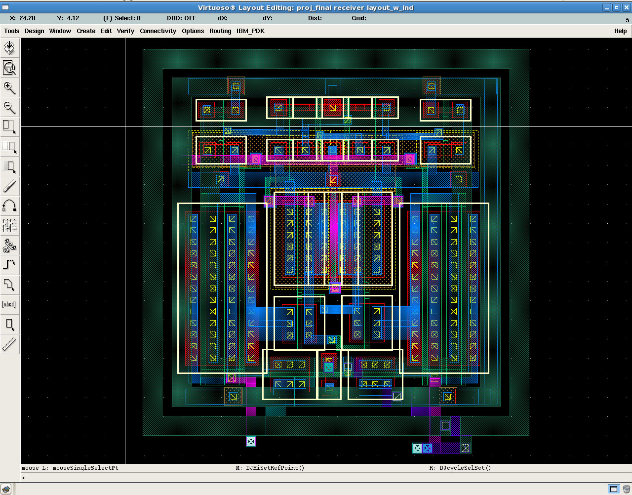
Layout of an RF circuit in a 0.13um CMOS process using Virtuoso.
Setup Cadence Environment
You must do this before running Cadence, and you only need to do this once.
- Login to a CAEN Linux machine in one of the CAEN labs. To connect remotely from a Windows computer or personal computer, login remotely to login.engin.umich.edu.
-
Authenticate using gettokens and your Kerberos
password. Create a link from your home directory to your EECS
311
AFS space. Replace <uniqname> with your UMICH
uniqname. If your directory does not exist, contact the course staff.
>> gettokens
>> cd ~
>> ln -s /afs/umich.edu/class/eecs311/f09/students/<uniqname> eecs311 -
All your Cadence files should be saved on the afs file server. You can
easily access this space from your home directory using the link you
just created.
>> cd ~/eecs311
-
Copy all of the the setup files to your afs space.
>> cp /afs/umich.edu/class/eecs311/f09/cadence/setup_working_dir/* ~/eecs311
>> cp /afs/umich.edu/class/eecs311/f09/cadence/setup_working_dir/.* ~/eecs311 -
For those who have used Cadence in a class before,
check your home directory for the following 2 files:
~/.cdsinit and
~/.cdsenv. If they exist, rename them
to ~/.cdsinit.tmp and
~/.cdsenv.tmp. Also remove any
Cadence-related modifications you made to your
~/.cshrc
file. The default .cshrc file can be found at /usr/caen/skel/std.cshrc.
Note: if you created these files for a class you are currently taking, you will have to undo these operations before launching Cadence for this other class.
Launch Cadence and Create a Library
- Login to a CAEN Linux machine in one of the CAEN labs. To connect remotely from a Windows computer or personal computer, login remotely to login.engin.umich.edu.
-
Launch Cadence from your afs directory. The Command Interface Window
(CIW) will pop up.
>> cd ~/eecs311
>> gettokens
>> icfb & -
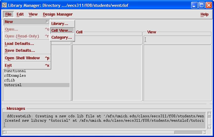
Next launch the library manager to create a new library by selecting
Tools > Library Manager... from the CIW.
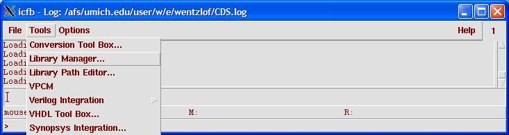
Launch Library Manager from the Command Interface Window (CIW). -
The EECS311Lib and EECS311Examples
libraries should appear in the Library Manager. Select
File > New > Library... from the Library Manager to create a new
library.
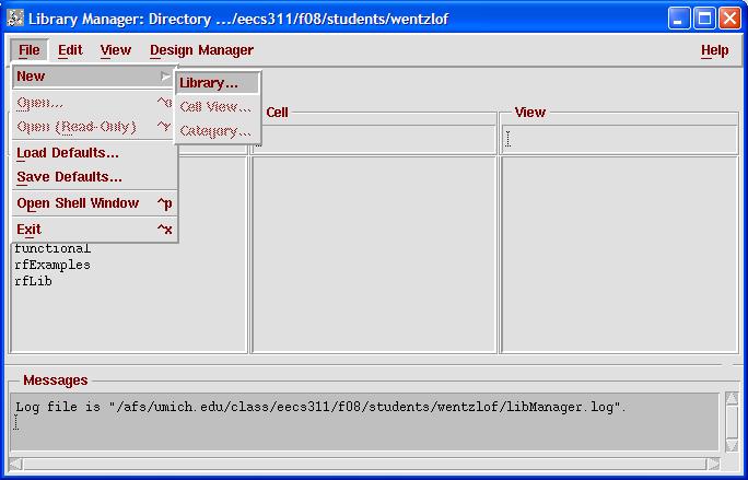
Create a new library. -
Enter tutorial for the Library Name and
click OK.
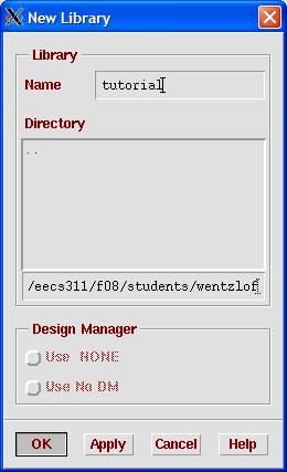
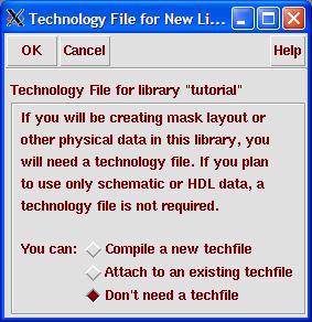
Create a new library. -
Select Don't need a techfile and click
OK.
Create a new library. - The library tutorial will now appear in the Library Manager.
Create a Schematic
- Launch Cadence and
open the Library Manager. Click on the
tutorial library in the Library Manager to select it, then go to
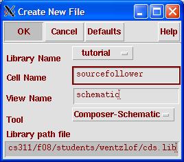
File > New > Cell View...
Open the create new cell view dialog box. - Enter sourcefollower for the Cell Name,
and choose Composer-Schematic for the
Tool. The View Name will automatically default to schematic. Click
OK.
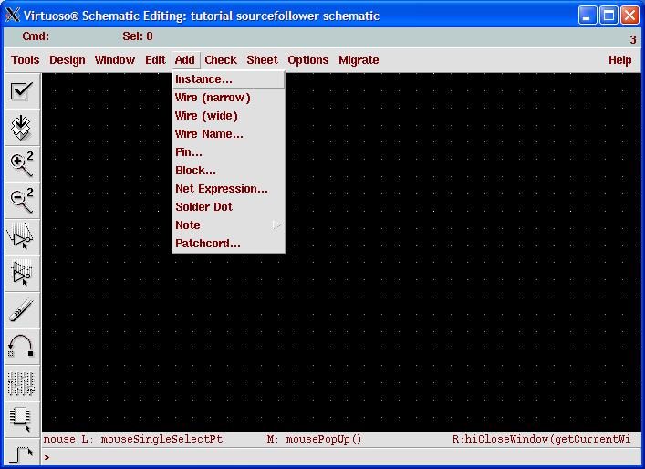
New cellview dialog box. - The new schematic will open up. To add a part to the schematic, go
to Add > Instance...
Schematic editor. - To find a part, click Browse from the
Add Instance dialog box.
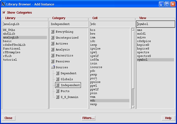
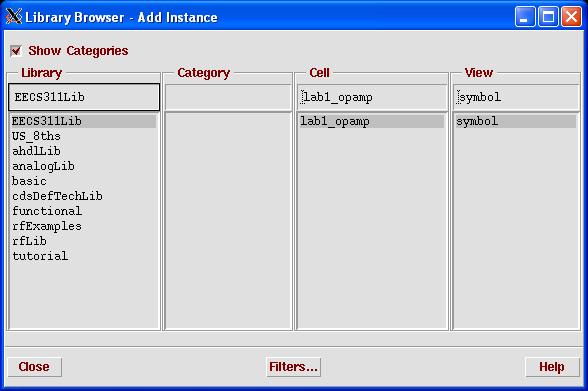
Add instance dialog box. - The Library Browser will pop up. First add a DC power supply. To
do this, select the analogLib library, the
Sources > Independent Category, the
vdc Cell, and the
symbol view. Click Close.
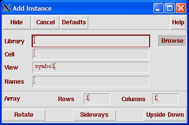
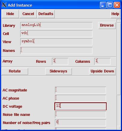
Library browser for finding parts. - The Add Instance dialog box will be populated with the vdc component
and fields for the component will appear at the bottom. Enter
12 for the DC voltage.
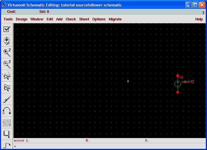
Add Instance dialog with vdc part populated. - Go to the schematic window and click to place the vdc instance as
shown below. Then hit the Esc key or click
Cancel in the Add Instance dialog.
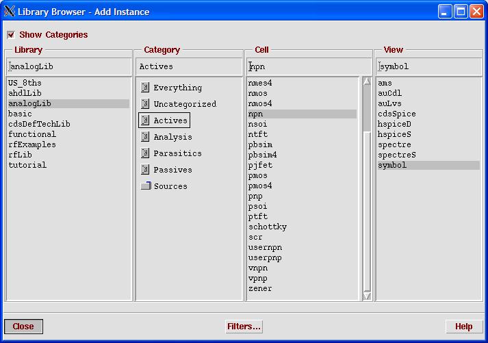
Schematic with vdc part placed. - Next add an NPN device. From the schematic window,
Add > Instance...
and then Browse to bring up the Library
Browser. Select analogLib,
Actives, npn,
symbol. Click
Close.
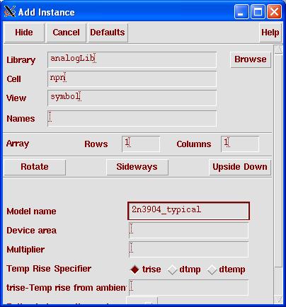
Library browser for finding parts. - In the Add Instance dialog box, enter
2n3904_typical
for the Model name.
Add instance dialog box. - Go to the schematic window and click to place the npn instance as
shown below. Then hit the Esc key or click
Cancel in the Add Instance dialog.
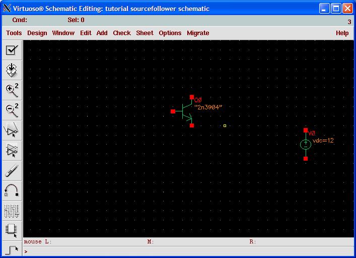
Place the npn device. - Next add a capacitor. From the schematic window,
Add > Instance...
and then Browse to bring up the Library
Browser. Select analogLib,
Passives, cap,
symbol. Click
Close.
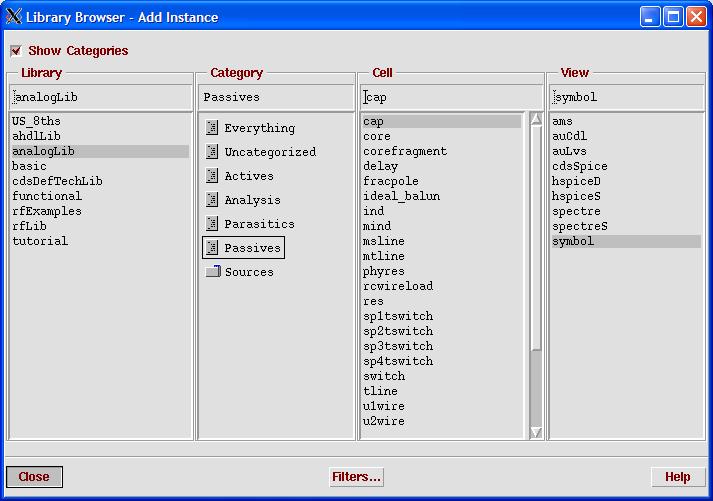
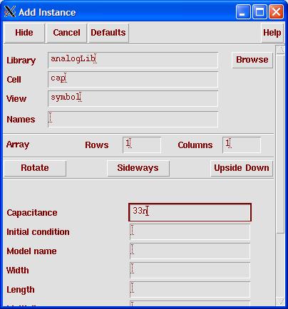
Library browser for finding parts. - In the Add Instance dialog box, enter 33n
(n refers to nano) for the Capacitance. Place the component on the
schematic. See also this link for other
units abbreviations
accepted by Cadence.
Add instance dialog box. - Go to the schematic window and click to place the cap instance as
shown below. Then hit the Esc key or click
Cancel in the Add Instance dialog.

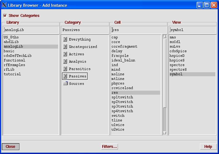
Place the cap device. - Next add 2 resistors. From the schematic window,
Add > Instance...
and then Browse to bring up the Library
Browser. Select analogLib,
Passives, res,
symbol. Click
Close.
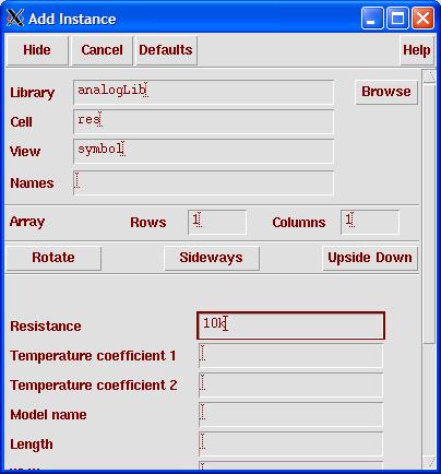
Library browser for finding parts. - In the Add Instance dialog box, enter 10k
(k refers to kilo) for the Resistance. Place the component on the
schematic. See also this link for other
units abbreviations
accepted by Cadence.
Add instance dialog box. - Go to the schematic window and click to place the 10k res instance
as shown below.
Place the res device. - To add the 1k resistor, back in the Add Instance dialog, change the Resistance value to 1k, and place the 1k res on the schematic. Then hit the Esc key or click Cancel in the Add Instance dialog.
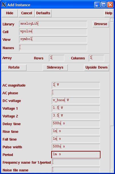
- Next, add an input source. From the schematic window, Add > Instance... and then Browse to bring up the Library Browser. Select analogLib, Sources > Independent, vpulse, symbol. Click Close.
- In the Add Instance dialog box, fill out the fields as shown below.
See this link for
units abbreviations accepted by Cadence.
Add instance dialog box. - Go to the schematic window and click to place the vpulse instance as
shown below.
Place the device. - Finally, place ground symbols on the schematic. Bring up the Add
Instance dialog box, and directly type in
analogLib, gnd,
symbol without bringing up the Library
Browser. Place the grounds on the schematic and hit
Esc.
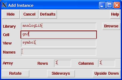
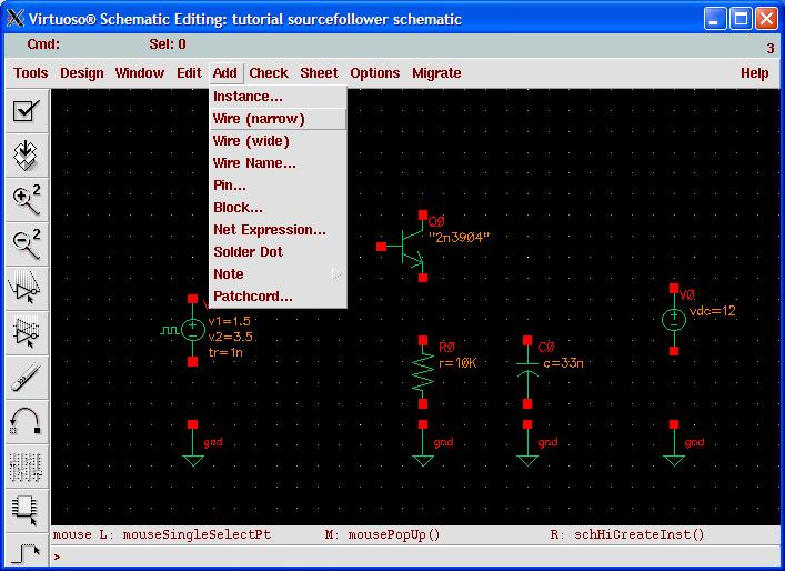
Add instance dialog box. - Add > Wire (narrow) and
single-click on the components pins to wire
up components.
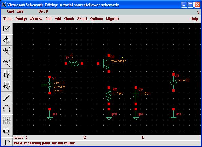
Add wires. - Wire up the schematic to look like this. After wiring all
components, hit the Esc key to cancel
adding wires.

Completed schematic. - Add > Wire Name... to name the nets.
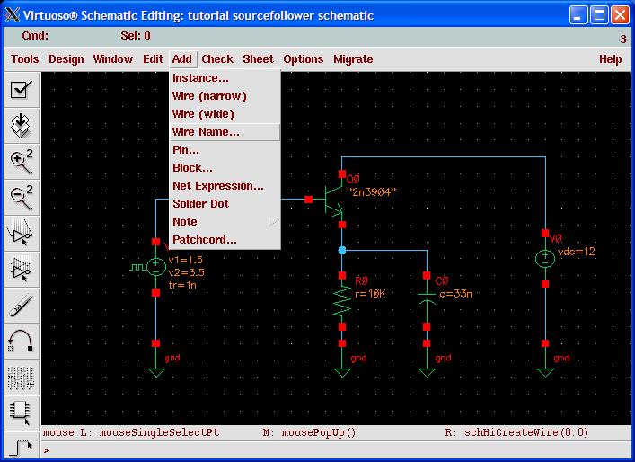
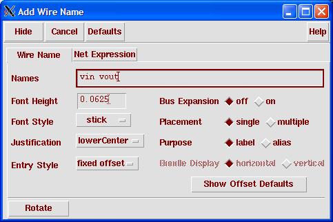
Adding wire names. - In the Add Wire Name dialog, enter the net names separated by
spaces. Type vin vout in the Names field
(note the space separating the names).
Add Wire Name dialog box. - Left-click on the input net first, and
then left-click output net to place the
wire names.
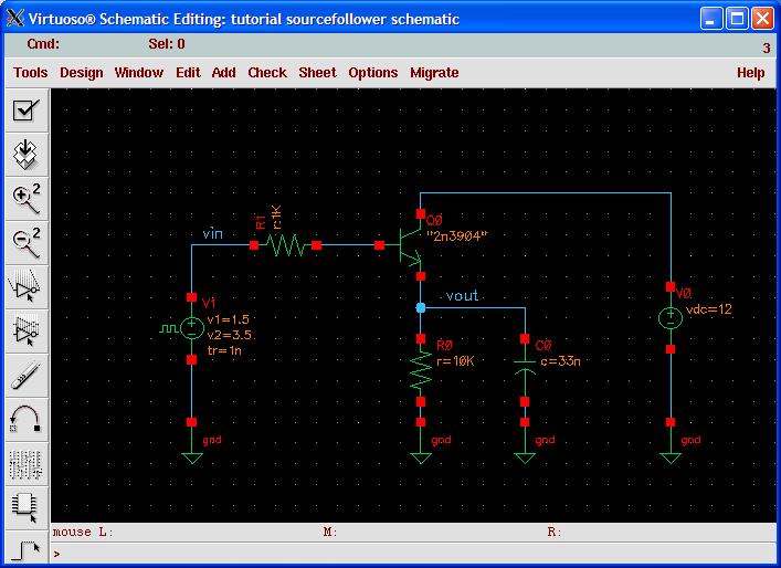
Schematic with net names. - To save the schematic, click on Check and Save
button in the upper-left corner of the schematic window.
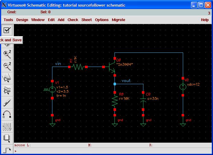
Check and Save the schematic.
Create a Schematic with an LM741
- Launch Cadence and
open the Library Manager. Click on the
tutorial library in the Library Manager to select it, then go to
File > New > Cell View.... Enter
741invertingamp for the Cell Name, and
choose Composer-Schematic for the Tool.
The View Name will automatically default to schematic. Click
OK.
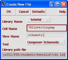
New cellview dialog box. - From the schematic window, Add > Instance...
and then Browse to bring up the Library
Browser. Select EECS311Lib,
lab1_opamp,
symbol. Click
Close.
Browse for the 741 opamp. - Place the opamp on the schematic.
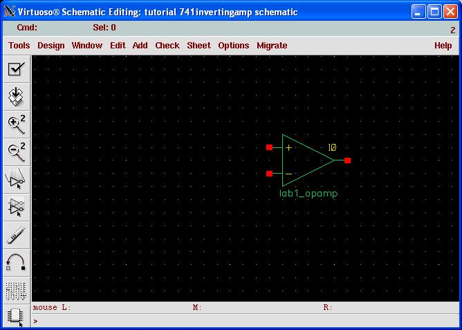
Schematic with opamp. - Using the Add > Instance... command,
add a 1kOhm and 10kOhm resistor (analogLib > res),
a sine wave input (analogLib > vsin), and
ground symbols (analogLib > gnd). Place
them as shown in the figure below. Use the Add > Wire Name...
command to name the vin,
vout, and vfb nets as shown below. Finally,
click the Check and Save button in the upper left
corner of the schematic window.
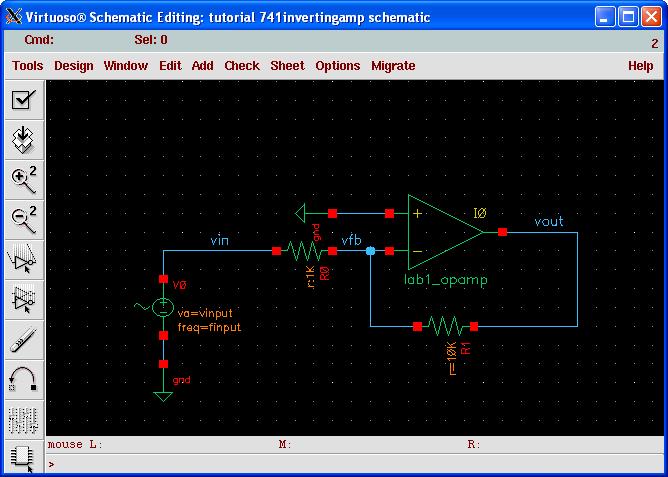
Final schematic with components and wire names.
Launch Analog Environment Simulator
- Launch the simulator, called Analog Environment,
from the schematic window by selecting Tools > Analog
Environment.
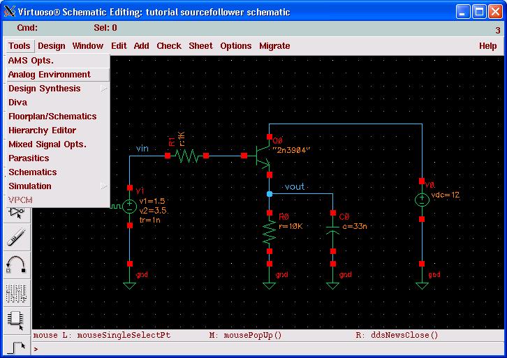
Launch Analog Environment. - The Analog Environment window will appear.

Analog Environment.
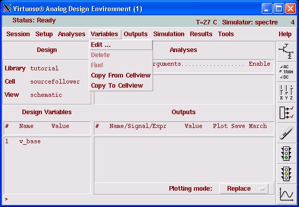
Load Variables
- Load any variable names from the schematic by selecting
Variables > Copy From Cellview.

Load variable names from the schematic. - Select Variables > Edit ... to edit the variable
values.
Bring up variable value editor. - The variable v_base was used in the
sourcefollower example as a DC bias voltage. Set this to 2.5V
by selecting the v_base variable in the righthand list,
entering 2.5 in the Value (Expr) field, click
Change, then click OK.
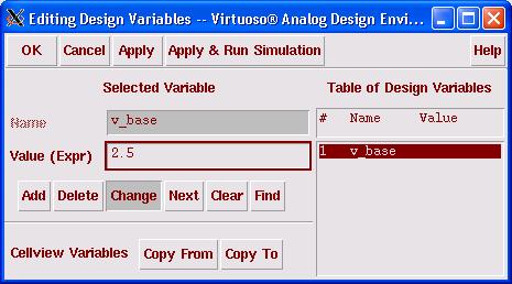
Changing the value of a variable.
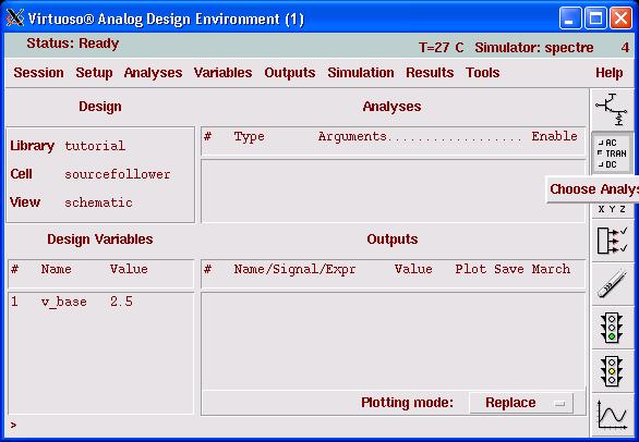
Simulating DC Operating Point and DC Sweep
- Click the Choose Analysis button on the righthand
side of the Analog Environment window.
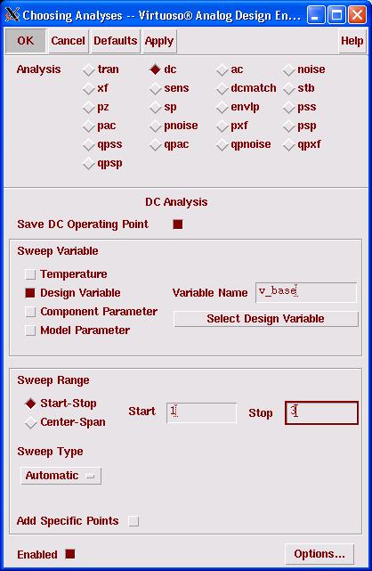
Click choose analysis. - Select dc as the Analysis type, select Save
DC Operating Point, select Design Variable as
the Sweep Variable, enter v_base in the Variable Name
field, enter a start and stop value of 1 and 3
in the sweep range to sweep v_base from 1 to 3 volts. Click
OK.
DC analysis configuration. - To run the simulation, click Netlist and Run in the
Analog Environment window.
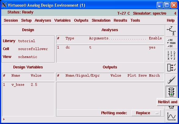
Click netlist and run to run a simulation. - To print the DC node voltages at the DC operating point, select
Results > Annotate > DC Node Voltages.
Look at the schematic, the voltages will be annotated
on the schematic.
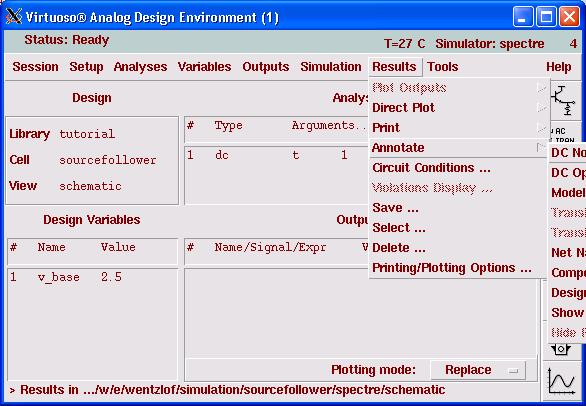
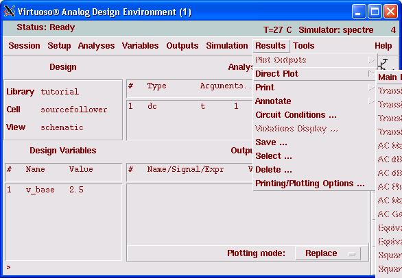
Annotate DC node voltages on the schematic. - To plot results from the DC sweep, select
Results > Direct Plot > Main Form.
Plot the DC sweep results. - Select the Function to plot, in this case, select Voltage.
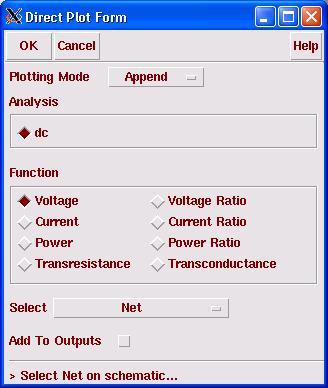
Plot the DC sweep results. - Switch over to the schematic window and left-click
on the vout
wire. A plot will automatically appear with the results.
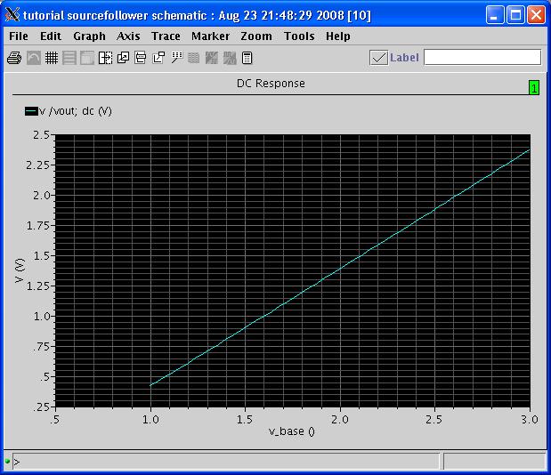
Plot the DC sweep results.
Simulating Transient Response
- Open the sourcefollower schematic and launch launch
Analog Environment using Tools > Analog Environment.
Select Variable > Copy from Cellview. Then use
Variables > Edit, select the v_base variable,
enter 5 in the Value (Expr) field, and click
Change. Click
OK.
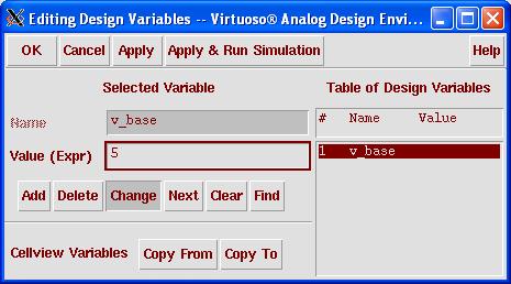
Change the value of v_base to 5. - From Analog Environment, click the Choose Analysis
button on the righthand side of the Analog Environment window. In the
Choosing Analyses dialog, select the tran Analysis,
enter 2m as the Stop Time, and check the
conservative box. Click OK.
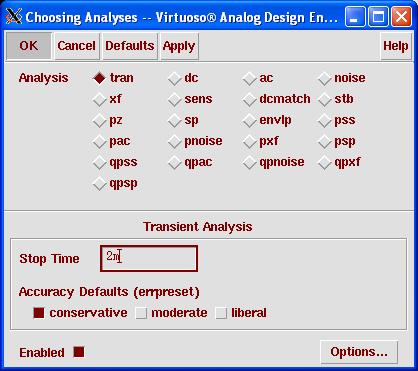
Transient analysis setup dialog. - Back in the Analog Environment window, click the Netlist and
Run button.
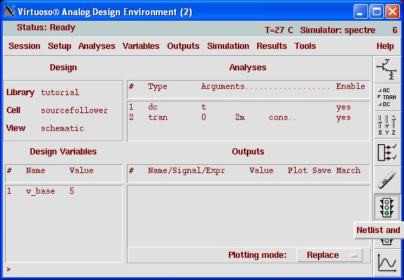
Netlist and run the simulation. - When the simulation completes, select Results > Direct Plot
> Main Form.... From this dialog you can plot various results.
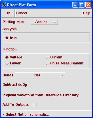
Direct Plot > Main Form dialog box. - With the Results > Direct Plot > Main Form... still
open, switch over to the schematic and click on the vout net.
This will bring up a plot window showing the output waveform. Continue
to click on nets to add plots to the graph. Hit Esc or
Cancel in the Main Form dialog to cancel plotting.
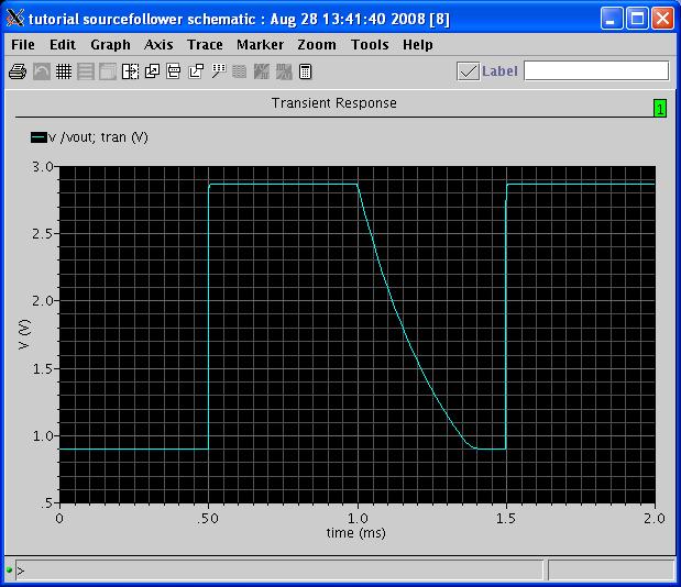
Transient output waveform.
Simulating AC Response
- Open the sourcefollower schematic and launch launch
Analog Environment using Tools > Analog Environment.
Select Variable > Copy from Cellview. Then use
Variables > Edit, select the v_base variable,
enter 5 in the Value (Expr) field, and click
Change. Click
OK.
Change the value of v_base to 5. - Click the Choose Analysis button on the righthand
side of the Analog Environment window. In the Choosing Analyses dialog,
select the ac Analysis, select
Frequency as the Sweep Variable, enter 1k as
the Start Stop Time, and check the conservative box.
Click OK.
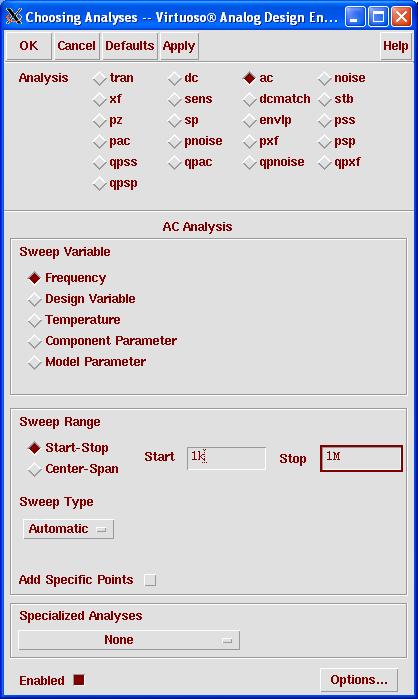
Transient analysis setup dialog.
Using Cadence from a Windows Computer
- Download and install Xming and Xming-fonts (you need both for Cadence). This is free X-hosting software for Windows.
- Download Putty. No installation is required. This is a free SSH client with X11 forwarding capability.
- Launch Xming. Once running, the Xming
icon will appear in the system tray.
Xming system tray icon (big X). - Launch Putty (Xming needs to be running
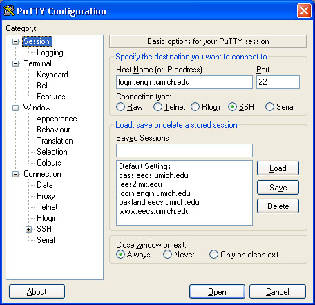
before logging in with Putty). Enter
login.engin.umich.edu in the
Host Name (or IP address) field.
- Click on the Connection > SSH > X11
Category, and check the box for Enable X11
forwarding.

- Click Open and login with your UMICH credentials.
Available EECS311 Device Models
The following models are automatically loaded into your environment and available for use after following the instructions to Setup Cadence Environment.
| Cadence Component | Model Name | Source | Description |
| AnalogLib > npn | 2n3904_typical | Fairchild | 2N3904, NPN, Beta=300, TO-92 Package |
| AnalogLib > pnp | 2n3906_typical | Fairchild | 2N3906, PNP, Beta=300, TO-92 Package |
| AnalogLib > nmos | 2n7000_typical | Custom | Simple NFET based on 2N7000, Vth=2.1V |
Units Abbreviations Accepted by Cadence
When entering numerical values into fields in the Cadence environment, you can use the following abbreviations for units. For example, to specify 0.1μF, type 0.1u or 100n. For 1MHz, type 1M or 1000k.
| Units | Abbreviation |
| Mega- | M |
| Kilo- | k |
| milli- | m |
| micro- | u |
| nano- | n |
| pico- | p |
| femto- | f |