|
Inertial Measurement Algorithm
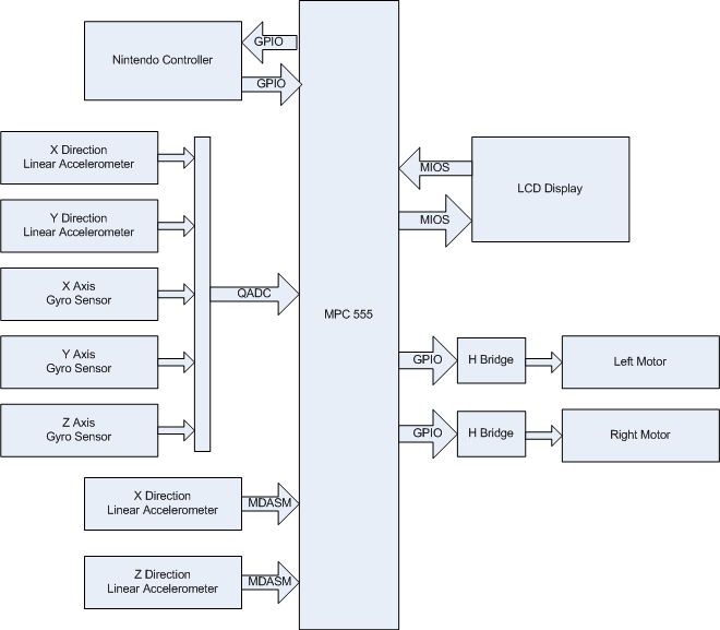
The data available to the robot from the sensors include acceleration data in three orthogonal directions (forward, right, up) and rotational velocity data around the same 3 axes. At a very basic level, any algorithm that uses this data to track position and heading would need to first perform some type of filtering to reduce the effect of noisy data. This data must then be translated from the robot's relative coordinate system to a global coordinate system that does not change as the robot moves. Finally, the acceleration data needs to be integrated over time in order to get the current position and angle measurements.
Our original approach was to use a Kalman filter to fuse the sensor data and get the position and angle measurements. Kalman filtering takes advantage of stochastic processes to filter out noisy sensor data, producing an estimate for system variables that were not directly measured (e.g tilt angle when you are measuring rotational velocity). It involved a computationally complex algorithm in which the processor would constantly make a prediction of all the system variables, would look at the sensor measurements and see if they were consistent with the state variable prediction, and then it would correct the predicted state variables using knowledge of the error covariance data between all the sensors and state variables. We developed a full program of this algorithm to run on the MPC555 chip. However, when updating the state variables at a 75 Hz rate the Kalman algorithm used about 85% of the CPU resources. Through research and testing we determined that 75 Hz was not fast enough to ensure reliable calculations from the sensor data. Instead an update rate of around 300 Hz seemed to give the best data. Also, using 85% of the system resources left little time to do other necessary tasks such as interfacing with the Nintendo controller or the LCD. For this reason we decided to not use the Kalman filter in favor of a simpler algorithm which we could run at a faster rate.
We began by looking at a smaller set of data. By ignoring tilt and z direction acceleration we could look at data from only 3 sensors, the forward and right acceleration and the rotational velocity about the axis go up and down. To lightly filter out some of this noisy data we would take an average of 3 sensor measurements as inputs to the algorithm. We then used heading angle to normalize the acceleration data to a global coordinate system. A single integration was performed on the rotational velocity in order to obtain the new heading and a double integration was performed on the acceleration data in order to obtain a new position. These integrations were performed through a Riemann sum since our data was discrete and not continuous.
An issue that we faced with these algorithms was the integration of any error introduced by our sensors. For example, when the robot begins moving at a constant velocity and then stops we will measure a positive acceleration at the beginning of the movement and then a negative acceleration at the end of the movement. If the integration of both of these acceleration humps don't perfectly cancel each other out we will be left with a non-zero velocity which will constantly be integrated into our position values throwing our accuracy off at an exponentially increasing rate. To remedy this we made the assumption that our robot would not be moving while being driven. Whenever the robot would stop we would zero out all of the velocity values to ensure that there was no drift due to slightly off acceleration measurements. We would also recalibrate the zero value of the sensors. As the robot moved around the zero value of the sensors would drift around, so this constant recalibration was necessary.
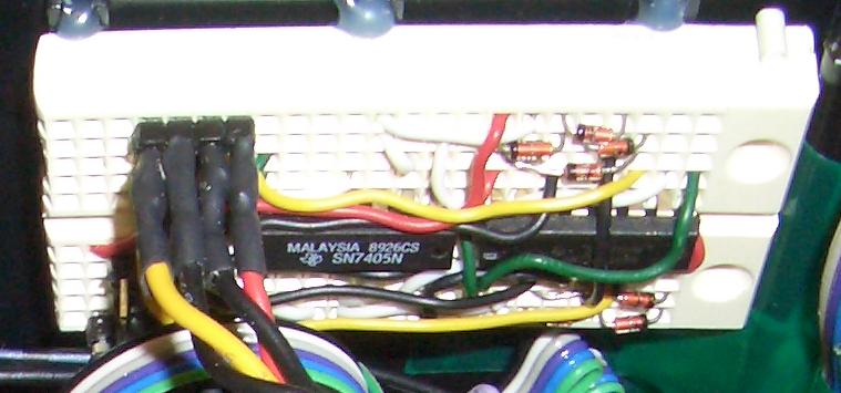
Sensors
The robot contained two analog accelerometers, three analog gyro sensors, and two PWM accelerometers. Although in the final version of our robot we used only the two analog accelerometers and one analog gyro sensor, we connected and programmed for all of these sensors. Through the serial debug interface we could access all of the sensor data and calibrate them all accordingly.
Built into the MPC555 were 10 bit queued analog to digital converters (QADC). To use this subsystem we had to set a queue of specialized QADC instructions that would tell the QADC various things such as what pin to sample the analog value from, how long to spend converting, and the alignment of the digital output. We set the QADC's to continuously scan all of the analog sensors three times without setting an interrupt and to store these values into an output queue of digital values. This allowed us to grab the latest analog data whenever the update algorithm required it without having to wait for the QADC's to sample. Each sensor was sampled three times so that we could take these three values and average them out to reduce noise.
In hardware we were able to set the voltage window within which the QADC would measure. We set this window from 0 to 5 volts. We did this because this was the range of our sensor with the highest voltage. Two of the sensors, the gyro sensors that measured tilt and not heading, gave output voltages from 0 to 3.3 volts. The resolution of this range when measured as a 5 volt range sensor was poor and gave us data that appeared really insensitive. To deal with this we built an amplifier circuit that used an op amp chip to scale the 3.3 volt range to a 5 volt range so that we could use the full range of the sensor using our QADC's. Since these sensors were not used in the final robot algorithm these amplifiers were not integrated into the final robot.
To measure the PWM inputs from the digital accelerometers we made use of the MPC555's MIOS Double Action Submodule (MDASM). We configured this device to input a free running counter. Whenever the PWM signal would go high, the MDASM would latch the counter value into an internal register, and when the PWM signal would go low it would latch the counter into a different register. It would also move the value from the first register to a new register whenever the signal fell. This allowed us to get reliable PWM measurements regardless of the phase of the signal. Whenever we wanted to sample the PWM measurement we could just look at the values of the registers with the latched in counter values and take the difference.
Periodic Interrupt Timer
The timing of the update algorithm was crucial to maintain in order to ensure the accuracy of the calculations. To maintain this timing we put the update algorithm into an interrupt routine that was triggered by the periodic interrupt timer (PIT). The PIT is a continuously running counter that can be configured to have different clocks and reset values. Whenever the PIT hits 0 an interrupt is thrown. By adjusting the prescaler value for the PIT input clock we could obtain a wide range of different interrupt frequencies. We configured our PIT to interrupt at a 300 Hz rate.
We also needed to be aware of how other algorithms were running relative to the update algorithm so that the other algorithms would not destroy the integrity of the data coming from the IMU algorithm. For example, the algorithm to update the graphics on the LCD was quite slow. If we interrupted the IMU algorithm with this LCD update function it would wipe out a lot of the sensor measurements and calculations. For this reason we put the LCD interfacing functions and the mode selection code into the PIT interrupt handler. This allowed us to tightly control the integration of the IMU algorithm with the other algorithms. For example, we could easily lock out the refresh of the LCD graphics when the robot was moving so that the sensor data would not get wiped out.
LCD Graphics Display
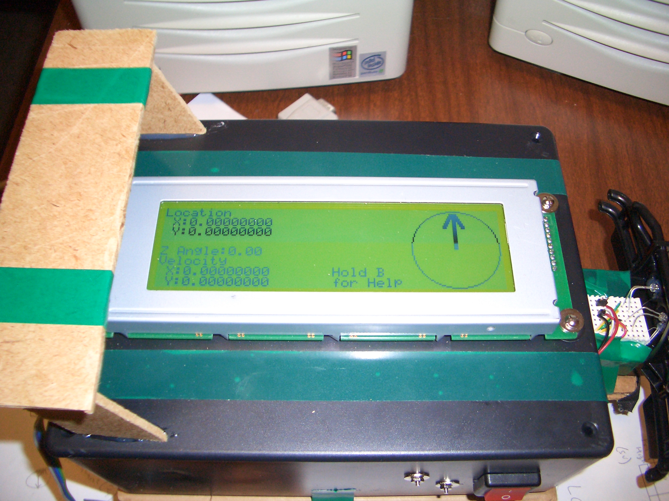
The display on the top of the Knightrider is an Optrex DMF5005 240x64 pixel graphics display. It has an internal Toshiba T6963 LCD controller that was interfaced to the MPC555 and controlled the refreshing of the LCD screen itself. In order to interface the MPC555 to the T6963, we had to implement a bidirectional data bus along with control lines for read, write, data/command, chip enable, and reset. Because we were using the MPC555 and did not have an FPGA, these lines were set up on the Modular Input/Output System (MIOS) built-in to the MPC555. Software control handled the setting of these lines.
|
An open source device driver for the T6963 that interfaced it to a PIC microcontroller was adapted to work with the MPC555. The bidirectional bus needed was set up by writing to the MIOS DDR (Data Direction Register). Writing a one to one of the bits in this register set that bit to an output, and writing a zero sets the bit to an input. By setting the control signals in the MIOS DR (Data Register) and reading or writing the data values to this register, the correct commands and data can be sent to the T6963. Problems that we came across while working with this display were making sure the correct initialization steps were followed, the LCD pins were connected to the proper MIOS pins, and adjusting the set/clear pixel functions to account for the fact that the 6x8 pixel font size had to be used for this display. Each byte of graphic memory only utilized 6 of the 8 bits for graphic data when using this font size.
|
|
After getting the initialization functions to work correctly, functions were then created to draw lines, circles, and arrows for the compass display. The text functions were used to display the vehicle's location, velocity and angle, and then the correct angle to point "home" was displayed on the compass display.
During vehicle operation, the text data is refreshed during the routine of the periodic interrupt timer. Because the graphics display must be cleared pixel by pixel and redrawn for a new compass, it only refreshes when the car is stopped. This ensures that the accelerometer calculations are not interrupted by the graphics display during operation.
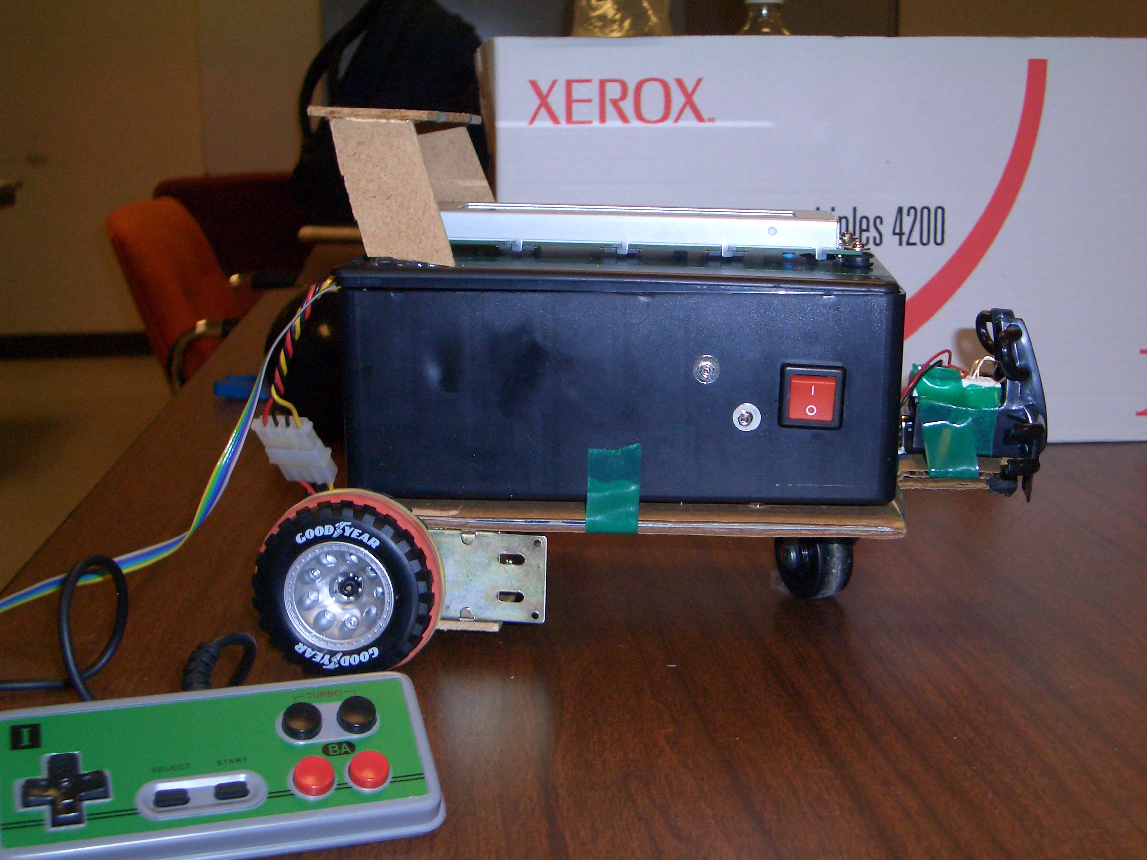
Nintendo 8 Controller
|
|
Implementing the Nintendo 8 Controller without an FPGA turned out to be pretty challenging. The controller has two input pins (latch and pulse) and one output pin (data). The user must send a short pulse on "latch" to trigger the 8-bit shift register to sample all the buttons. Then a series of pulses on "pulse" will shift the status of each button out to "data". In order to generate the two signals withough tying up the MPC555 by using a software counter, I decided to use the MPC555 Time Base Counter to generate appropriately spaced interrupts. In software, I essentially implemented a state machine that would cycle through the correct sequence of latch, eight pulses, and then a delay to cause a sampling rate of approximately 60 Hz. My code has a counter to guide it through a series of stages. Stage 1 brings Latch high, and sets the counter reference to 12 us. Stage 2 brings latch low, stores the value on the data line, and sets the counter reference to 6 us. Odd stages from 3 to 16 set pulse high, and even stages from 3 to 16 set pulse low, and records the value on the data line
|
into the corresponding array cell. Stage 17 sets the reference value to 1/60 Hz, and cycles back to stage 1. Latch, Data, and Pulse were configured through the USIU's GPIO pins. The Time Base Counter is also a part of the USIU.
Motor Control
Implementing the motor control system proved to be quite time consuming. We decided to use an H-Bridge chip (SN754410) that was provided to us by Matt Smith. Using a circuit design adapted from the data sheet, we found we were able to control speed and direction of the motors using only one PWM signal for each motor. The idea is simple enough... We implemented the H-Bridge in such a way that with a high signal the motor would spin forward, and with a low signal the motor would spin in reverse. Thus sending a PWM signal at a relatively low frequency (say 1kHz) we were able to easily control speed and direction simply by varying the duty cycle of the PWM control output. With this implementation
|
|
a 50% duty cycle would yield no movement of the motors. In order to conserve power, we also made use of a general purpose output pin to enable and disable the use of the control circuit. This allowed us to "shut off" the motors when they were set to a 50% duty cycle so as not to waste power.
Using this design, the software was written to control the PWM and enable outputs. For example, to drive straight forward, a PWM signal near 100% was sent to both motors. Since both the right and left motors had their own driver, we could adjust this function to accommodate for the fact that each motor was not identical. We simply adjusted each motors individual speed by varying the duty cycles to ensure that they had the same speed and the car would drive straight and not drift in one direction or the other. Likewise to turn, duty cycles near opposite sides of the percent spectrum were sent to each motor. Again, we calibrated the duty cycles of the PWM signals so be sure that the car would rotate about its center axis. This was important as we found that that it affected the accuracy of the position values that were read from sensors and filtering algorithms described above.
Auto-Pilot Algorithm
As described above, when the user decides that the robot should drive itself home, he can press the "Start" button on the Nintendo 8 controller and the robot will switch into "Auto mode" which runs our auto-pilot algorithm. The idea of the the autopilot can best be described in the following steps. First, the robot will calculate the angular direction in which it needs to be pointed in order to drive home. Next, if the robot is not pointing with in some tolerance range of said direction, then the robot should turn until it is. And finally, once the robot is pointing in the direction of its defined home, then it can drive forward until it either reaches home or determines that it needs to adjust its heading in which case it will again turn.
Some important things to note: While the robot is driving straight, it is constantly calculating and recalculating the current desired heading and comparing it to its current heading as read from the sensors. This ensures that the robot always drives in the correct direction. Should its heading drift away from the direction of home, then the algorithm will account for this error immediately. Also, we found that forcing the robot to pause driving for one second every two to three seconds, the accuracy of the auto-pilot increased. This was due to the fact that in forcing the robot to pause we were able to re-calculate the current position more accurately, and re-zero the accelerometers which limited any errors from being propagated and amplified any further in the algorithm.
|


