Control Theory
Feedback Control • PID Control • Signals & Filtering • Linear Time‑Invariant (LTI)
ENG100/400 — Lecture 5
Agenda
- Why control? Open‑loop vs closed‑loop
- Feedback control block diagrams and stability
- PID control: intuition, math, tuning
- Signals and filtering: time vs frequency, simple filters
- FIR vs IIR filters: structure, pros/cons, usage
- LTI systems: impulse response, convolution, state‑space
- Preview: interactive apps to be added in lec5/
Overview: What is a control system?
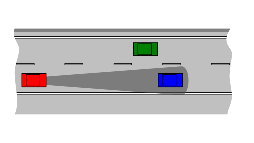
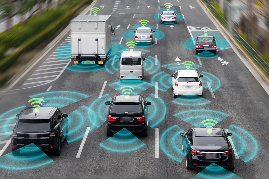
- A control system manages, commands, directs, or regulates the behavior of other devices or systems.
- Examples: self‑driving cars, temperature control, robots.
Why Feedback?
Open‑loop
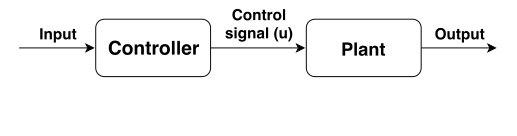
- No measurement of output
- Sensitive to disturbances and model errors
- Example: set motor PWM and hope for target speed
Closed‑loop (Feedback)
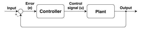
- Measure output and correct the input in real time
- Robust to disturbances, improves accuracy
- Example: speed controller measuring RPM and adjusting PWM
Effective control
Control system basics
- Plant: system to be controlled (e.g., car, room, robot)
- Control signal: input to the plant (e.g., throttle, heater)
- Output: state of the plant (e.g., speed, temperature)
- Controller: mechanism for controlling the plant (e.g., cruise control)
- Controller input: desired state (reference)

Control system types
Stability & Performance
- Stability: all closed‑loop poles in left half‑plane (continuous) or inside unit circle (discrete)
- Performance: rise time, overshoot, settling time, steady‑state error
- Robustness: maintain performance with disturbances and uncertainty
- Design trade‑offs: bandwidth vs noise; speed vs overshoot
PID Control
Control law (time domain): $u(t) = K_P e(t) + K_I \int_0^t e(\tau)\,d\tau + K_D \dfrac{de(t)}{dt}$
Intuition
- P: proportional to error — fast response
- I: accumulates error — zero steady‑state error
- D: predicts — damps oscillations
Implementation tips
- Use anti‑windup for I term (clamping or back‑calculation)
- Filter D term (e.g., first‑order low‑pass)
- Respect actuator limits; consider rate limiting
PID Tuning
- Ziegler–Nichols: increase Kp to ultimate gain Ku at sustained oscillation; Tu = oscillation period
- Then set $(K_P, K_I, K_D)$ from tables; refine by testing
- Practical: start with P only, add I for bias, add D to reduce overshoot
- Always validate with step tests and disturbance rejection
Signals & Filtering
- Sampling: $f_s$ must exceed 2× the highest signal frequency (Nyquist)
- Aliasing: high‑frequency content folds into low frequencies — use anti‑alias filters
- Noise vs bandwidth: filtering reduces noise but adds delay
- Common filters: moving average, exponential smoothing, RC low‑pass, notch, Kalman (model‑based)
FIR vs IIR Filters
FIR (Finite Impulse Response)
Difference eq: $y[n]=\sum_{k=0}^{M} b_k\,x[n-k]$
- Always BIBO stable (no feedback)
- Can achieve exact linear phase (symmetric $b_k$)
- Often needs higher order for sharp roll‑off
IIR (Infinite Impulse Response)
Difference eq: $y[n]=\sum_{k=0}^{M} b_k\,x[n-k] - \sum_{m=1}^{N} a_m\,y[n-m]$
- Uses feedback: efficient, sharp responses with low order
- Must ensure stability (poles inside unit circle)
- Nonlinear phase; may need phase compensation
Choosing between FIR and IIR: consider stability guarantees, phase requirements, computational budget, and latency.
Simple Filter Examples
Moving average
$y[n] = \dfrac{1}{N} \sum_{k=0}^{N-1} x[n-k]$
Great for smoothing; adds group delay of about (N−1)/2 samples.
First‑order low‑pass
Continuous: $\tau \dot y + y = x$ → Discrete: $y[n] = \alpha x[n] + (1-\alpha) y[n-1]$
Choose $\alpha = 1 - e^{-T_s/\tau}$ for sample time $T_s$.
Simple Filter: Numeric Input Demo
Compare EMA (IIR) and finite moving‑average (FIR). Use manual input or simulate random data to see differences.
Tips: Try an impulse (0,0,1,0,0,…) or a step (0,0,1,1,1,…). Use Sweep to see how FIR window length affects lag vs smoothness.
| n | x[n] | EMA | FIR |
|---|
LTI Systems
- Linear: superposition holds; Time‑Invariant: properties do not change with time
- Examples: mechanical and electrical systems (without hysteresis)
- Characterized by impulse response h(t) (or h[n])
- Output is convolution: $y = x * h$
- Frequency response: $H(j\omega)$ or $H(e^{j\omega})$ via Fourier/Z‑transform
State‑Space Form
Represents an LTI system assuming constant coefficients
Continuous: $\dot x = A x + B u, \quad y = C x + D u$
Discrete: $x_{k+1} = A_d x_k + B_d u_k, \quad y_k = C_d x_k + D_d u_k$
- Poles = eigenvalues of A (or Ad); controllability/observability guide design
- Enables modern design: LQR, observers (e.g., Kalman filter)
Interactive Apps
Explore these standalone demos under lec5/:
- PID step response and tuning
- Filtering and aliasing visualizations
- LTI convolution and frequency response
Tip: Open in a new tab. You can return here with Alt+Tab or your browser back button.
Open‑Loop Cruise Control
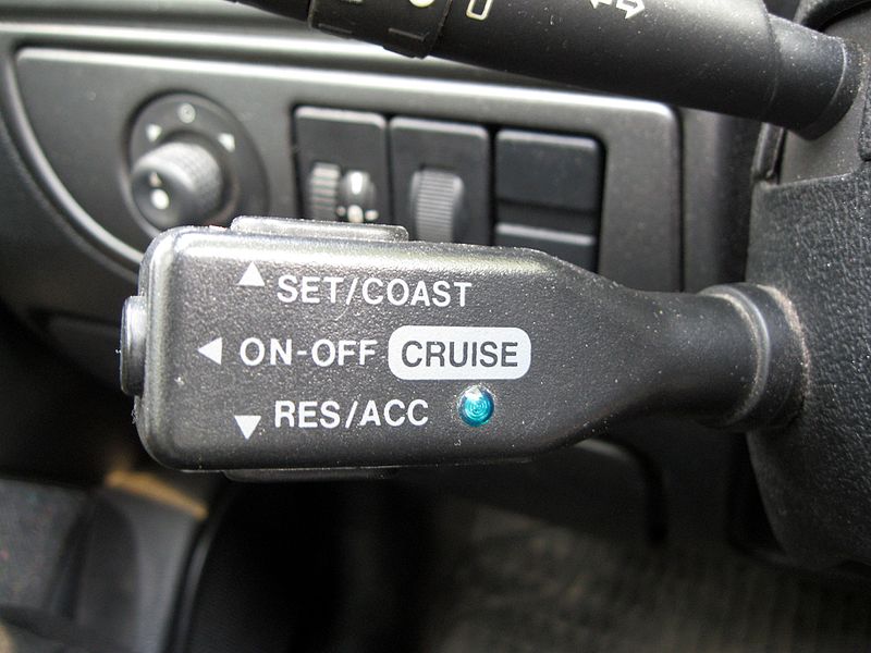
Source: wikimedia.org
Achieving a target speed
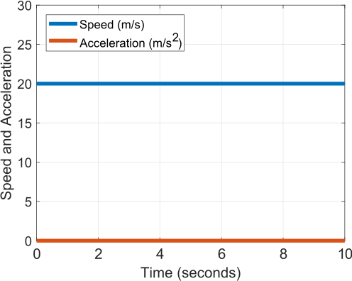
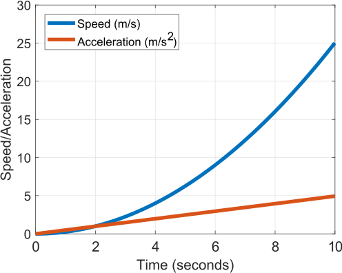
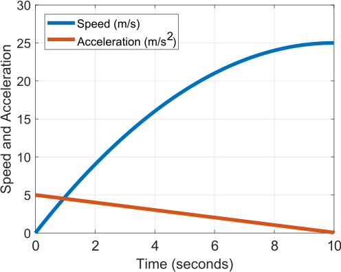
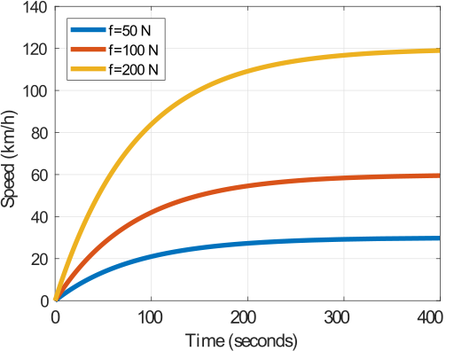
- Assume we can directly control force exerted on the vehicle.
- Try to reach target with a constant force.
Open‑Loop: Newton's law
Force = Mass × Acceleration. Using small Δt, a(t) ≈ (v(t+Δt) − v(t)) / Δt.
Open‑Loop: Model and steady‑state
Total force: $f - d - \alpha v(t) = m v'(t)$. Solution: $v(t) = \tfrac{f - d}{\alpha} + c_0 e^{-\alpha t/m}$.
Steady‑state: $v_\infty = \tfrac{f - d}{\alpha}$. To reach $v^*$ in steady‑state, choose $f = \alpha v^* + d$.
Closed‑Loop: Proportional control
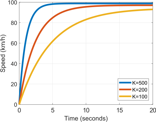
Control law: $u(t) = K e(t)$, here $f(t) = K (v^* - v(t))$
Speed under P control (for $v_0=0$):
$v(t) = \dfrac{K v^* - d}{K + \alpha}\big(1 - e^{-(K+\alpha)t/m}\big)$
Closed‑Loop: Toward PID
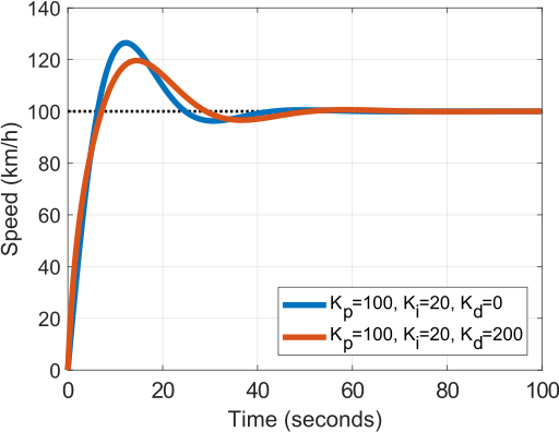
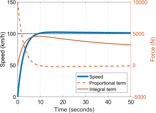
$u(t) = K_p e(t) + K_i \int_0^t e(t)dt + K_d \dfrac{de(t)}{dt}$
- Add I: eliminate steady‑state error
- Add D: anticipate changes and add damping

Closed‑Loop: PI and PID responses
MATLAB code: Closed‑loop examples
Excerpt from 03 Control/matlab/closed_loop_control.m
% Plant and P controller
m = 500; alpha = 6; v_target = 100; t = linspace(0, 20, 1000);
P = tf(1, [m, alpha]);
Kp = [500, 200, 100];
for i = 1:length(Kp)
  C = pid(Kp(i)); T = feedback(C * P, 1);
  v = v_target * step(T, t);
end

% PI contributions and PID comparison
Kp = [100, 100]; Ki = [20, 20]; Kd = [0, 200];
for i = 1:length(Kp)
  C = pid(Kp(i), Ki(i), Kd(i), 2); T = feedback(C * P, 1);
  v = v_target * step(T, t);
end
Wrap‑Up
- Feedback closes the loop for robustness and accuracy
- PID is a versatile baseline controller
- Filtering and sampling fundamentals matter for real sensors/actuators
- LTI framework unifies time and frequency‑domain analysis