Basic Lab Instrument Operation
Each work station is equipped with a set of basic lab instruments that
you will use in conjunction with the microprocessor development system
tools. Each station has an MSO (mixed signal oscilloscope),
signal generator, digital multimeter and triple output power supply.
The lab also has several portable USB based 8 channel logic analyzers
that you can check out of the lab for project work at home or other
purposes.
The Mixed Signal
Oscilloscope (MSO)
Each work station is equipped with a Agilent MSO-X 3012A mixed
signal oscilloscope. This is probably the most useful and complete
instrument on the workstation. The MSO-X is capable of observing 2
analog signals and 16 digital signals simultaneously. So it can behave
like a
basic analog signal scope and 8 channel logic analyzer. It also has a
fairly good signal generator and digital voltmeter built in too.
For starters, we will just use the scope to observe some simple analog
signals. In the following section we will observe a basic sine wave
generated from the signal generator so you can get a quick introduction
to each instrument.
For more detail on the scopes operation, you should try the following
exercises in the Agilent's training guide manual at Training
Guide.
- Exercise 1) Lab #1:
Making Measurements on Sine Waves
- Exercise 2) Lab #2:
Learning the Basics of Oscilloscope Triggering
- Exercise 3) Lab #4:
Documenting and Saving Oscilloscope Test Results (Taking screen shots)
It is not necessary to do this in the lab today, but you should
consider coming into lab when you have some free time to run through
them. Of course, reference the manual as need be. The scope also has an
excellent help function. Simply push the help key (lower left) and you
will be provided instructions.
In-Lab Part 4: Observing a Sine Wave
with the Oscilloscope
Step 1: Agilent 33220A Waveform
Generator Setup
Next we will use the Waveform generator to generate a sine wave and
view it
on the scope. First turn on the Waveform generator with the power
button. Next,
select Utility, then System Output using the blue
buttons. Select
High Z for load and hit Done.
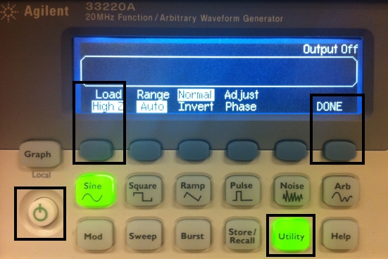
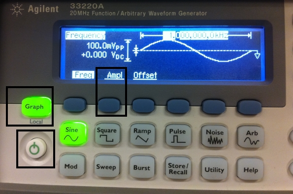
1.1) Next, hit the Graph
button. Then tap the Ampl button twice until it changes to HiLevel.
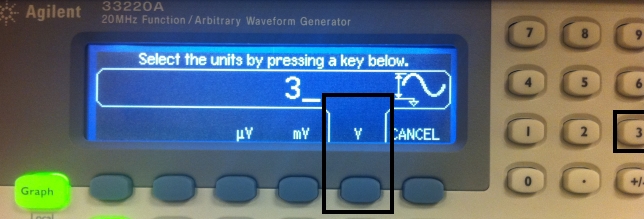
1.2) Next, select 3 V using
the number pad on the right and the blue button.
1.3) Finally, set the LoLevel
to 0 V using the number pad. Don't turn on the output yet.

Step 2: Settuing up the
Scope

2.1) Connect a three way BNC
adapter to the function generator. Connect one BNC cable to the scope's
channel one. Connect another one to the Red/Black
pin adapter, which will be used with the Logic Analyzer later. Now turn
on the Function Generator's output. Then hit Auto-Scale.
You should see the following trace.

2.2) This is a screen
shot from the scope. If you have a USB flash drive, you might
want to try saving. For this post lab and others you are asked to
provide screen shots.
2.3) Try Some Basic Triggering
Auto Scale will put the scope in Auto trigger mode or will cause the
scope to constantly trigger or display what is applied to the input.
Turn off the signal by toggling the signal generator OUTPUT button. You
should notice that the scope shows a flat line at the zero volts or
ground level.
Sometimes it is desirable to capture a single event. For the post lab
will observe the electrical signal that occurs as a consequence of
mechanical switch bounce. This a transient condition and will only be
available for short time. If we were to use Auto trigger mode the
display would soon replace transient condition with a steady state
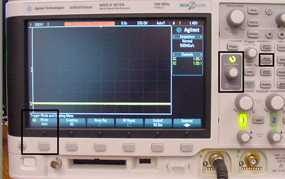
signal. We can capture the transient with the normal trigger mode. In the trigger
functions box, select Mode/Coupling. On the lower left you will see the
menu Mode Auto menu appear. Select with the soft key below. You can
choose the setting by rotating the Push to Selet Knob (center with grey
background) pushing to select.
Try turning the signal on and off again. You will see the sine wave
stays on the screen. This is because in normal trigger mode the
screen is not refreshed automatically. It is only refreshed when a
signal is present. In this way you can capture transients like the
switch bounce we will observe in the post lab assignment.
The Saleae Logic Analyzer
What is a Logic Analyzer?
Logic analyzers are used to verify logic
functions by observing logical signals as we did with the oscilloscope.
The
big difference is that you can observe many more signals with a logic
analyzer
then you can with a basic 2 channel scope. The problem is you
cannot observe the
signals with the same vertical (voltage amplitude) or horizontal
resolution
(time). The logic analyzer classifies and then stores the input
signal's
amplitude as either a high or low. The Saleae's maximum sample
rate
is 24MHz providing a time measurement resolution of about 0.1us.
Remember, with the scope we could resolve propagation delays
to about 1ns. Depending on the application, these measurement
resolutions are
tolerable when observing basic logic function and when time
measurements are
much greater than 0.1us.
Saleae Kit Installation
The Saleae DLA is powered via the USB connection, so simply plug it
in. Note: the analyzer does not work thru the display USB port.
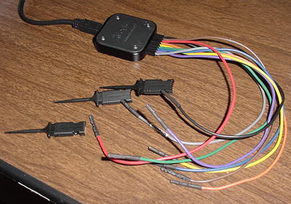
The analyzer is quite compact with one USB connection and a probe
pod consisting of 8 signal wires and a reference or GND connection.
Each probe has a socket connector on the probe end that be connected
into common circuit board headers or grabber clips supplied with the
kit.
Saleae Application Program
The Saleae application program can be evoked from the following
start menu ICON or from the program list.
A following window should appear.
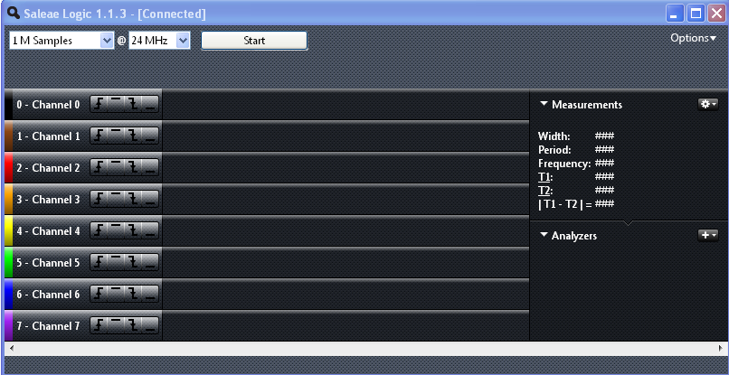
If the USB connection was successful, you should see a "Connected"
message in the upper window border. The first user drop down window
allows you to set the sample buffer size. Generally, 1 M samples
will do. The next window allows you to set the sample rate. For this
lab we will use the maximum rate providing a time resolution of about
01.us. The "Start" button starts a measurement. Note,
each channel is color coded to follow the probe color.
Simple Sampling
Give the analyzer a try by connecting it to the Signal
Generator. Provide a nice simple digital signal by changing the sine
wave to a square wave 1kHz, 3Vpp signal. Making sure that the
signal is 0V at it's lowest and 3V at it's highest rather than +/-
1.5V. Connect channel zero to the source output and don't
forget the ground reference. With the above setting take a sample by
hitting the "Start" button. You should see something like this.
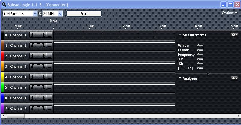
You can adjust the horizontal time scale by holding the mouse over the
waveform display area and scrolling up or down. Holding the mouse over
the waveform will provide a period, frequency and pulse width
measurement if they are enabled in the measurements window.
Notice that there is no vertical scale or voltage input gain
adjustment. The DLA displays the input signal as either a logical 0 or
1 in much the same manner as typical digital logic would interpret an
input signal. If the input value is -0.5V to 0.8V the value is
displayed as logical 0. If it is in the range 2.0V to 5.25V it is
displayed as logical 1. Values in between 0.8V and 2.0V can either be 0
or 1. Note you should take care not to exceed the input range
-0.5V to 5.5V when making measurements or you may damage the DLA input
circuitry.
Triggering the DLA
You will notice that if you take multiple samples of the
scopes 1kHz signal, the waveform will appear to shift or start at
different points in time. When you hit the start button, sampling
starts at different points along the waveform. Quite often we want to
trigger on a specific signal event much like we did with the
oscilloscope. A particular channel can be triggered for either rising
edge, falling edge, logical low or logical high level. The
conditions
are set with the 4 button set for each channel. To trigger the
channel 0 for rising edge, select the rising edge and hit
the
start button with the scopes 1kHz ref signal attached. The
display will look something like this.
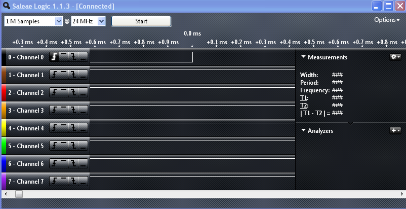
Notice that the display time base is now roughly centered at
0.0ms with time decreasing before and increasing after the 0.0ms time
marker. The 0.0ms marks
the trigger point. The signal is sample before and after the trigger
and stored in the sample buffer for observation about the trigger
point. You can adjust the display to see more waveform cycles.
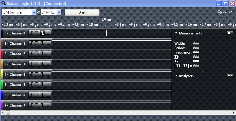
Selecting the negative edge likewise causes the trigger to occur
accordingly.
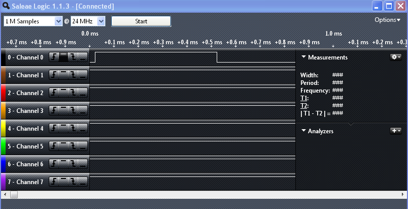
Likewise, triggering can be logical level 0 or 1 sensitive. This is
the display for a positive level trigger.
Triggering on Multiple Conditions
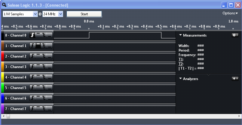
Sometimes we wish to trigger on more than one condition.
For
example, consider triggering on channel 0 with a rising edge and
channel 1 at a logical 1. You can attach channel 1
to the 3.3V test pin (near push button switch 2) on the SmartFusion
Kit. The
display will look something like this after a start measurement.
However, if we attach the channel 1 to the gnd pin next to the 3.3 volt
pin and we attempt to sample, the DLA will continue to monitor, but
wait for the trigger condition to come true before recording. The
following message will appear.
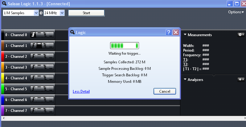
Move the probe to the 3.3 volt pin and you will see the DLA trigger.
Note, once
you lift the probe from the gnd pin the input will be interpreted as
logical
one
and the DLA will trigger.
Note, if you let the analyzer run long enough
at 24 MHz it may stall. It will report that the analyzer cannot sustain
the current sample rate. Simply hit the "Start" button again.
Observing a Sine wave with Logic Analyzer?
Connect the logic analyzer to the signal generator like so:
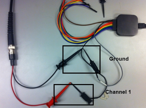
Switch the signal generator back to sine wave and observe the signal on
the logic analyzer. Be prepared to answer the following question
for the post lab: How does the sine wave look on the LA compare to the
square wave? Why if at all are they different?
More on the Saleae DLA
The Saleae DLA also has the ability to monitor and decode serial IO
protocols such as RS232 (UARTs), I2C and SPI. We will explore these
capabilities in later labs. Go to the Saleae website and read the
manual for more detail.
The MSO has all the digital functionality of the Saleae DLA, but we
will not cover that for present.
Measurements with the
Digital Multimeter and Lab Supply
Each workstation is equipped with an Agilent digital
multi-meter (DMM). The DMM is used for general measurements including:
voltage, current,
resistance
and capacitance. These should be relatively familiar to you from
introductory
lab courses.
For a simple application, let's measure the power
drawn by the kit. We
can model the kit as a load resistor for this measurement. By measuring
the
voltage across the kit and the current supplied we can determine the
power
load. Voltage to the kit is provided through the USB cable. We could
cut the USB cable to measure the power, but that would be just a tad
messy. Instead, let's use the lab power supply.
Set the Power Supply Output
Before hooking anything up, adjust the power supplies
6V output to be 5.00
volts. Note you have to have the Output turned on.
Connect the Kit to the Power Supply
Disconnect the USB cables from your kit. Get a BNC
cable, BNC grabber
adapter and BNC to banana adapter.
TURN
OFF THE POWER SUPPLY OUTPUT
TAKE
CARE TO CONNECT THE BANANA TO BNC CONNECTOR
WITH THE GND TAB ON THE GROUND TERMINAL OF THE POWER SUPPLY. FAILING TO
DO
THIS WILL APPLY NEGATIVE VOLTAGE AND FRY THE KIT!!

Next, connect the red clip to the kits 5 volt supply
test pin and the black
clip to a GND test pin.

Turn the power supply kit output on and you should be
able to observe the
current supplied to the kit. The power supply current meter is accurate
for
currents >10ma. Let's check it. Get another cable like the one you
used to
hook the power supply to the kit. Attach the cable to the DMM's current
terminals.

The adapter ground ref tab orientation is not
critical. It will only effect
the current flow reading direction (+/-). Next place this cable in the
ground
path of the power supply cable like this.

Observe the difference. At this current level the
power supply meter should
be very accurate. In most cases the power supply meter is adequate.