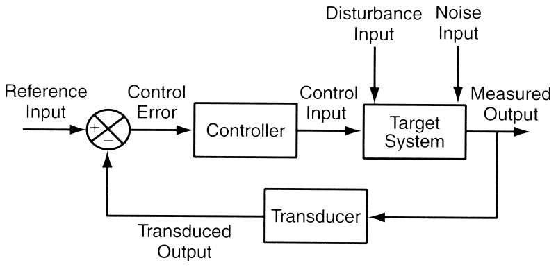
Basic block diagram of a feedback control system. The desired output value is specified with a reference input. The controller should adjust the setting of the control input to get the measured output to equal the reference input. (Figure from Feedback Control of Computing Systems, Joseph L. Hellerstein, Yixin Diao, Sujay Parekh, Dawn M. Tilbury)
The following plot is representative of a properly designed and adjusted control system. The horizontal axis represents time, in steps equal to the basic sampling interval of the system. The vertical axis represents the output value of the system. In this case, both the reference input (not shown) and the output start at zero. The reference input increases to 2 at time 50, and decreases to 1 at time 100. Note that after each reference input change, the output moves smoothly and quickly toward the desired new value.
This illustrates the properties of a good control system.
One common type of control system used a PID controller. With this type of controller, the control input is obtained from the control error by adding three terms:

Sometimes some of the constants are set to zero; not all terms are always used. For example, sometimes only the proportional term has a nonzero constant and the integral and derivative terms have constants set to zero (so they are not used at all). This type of controller is known as proportional control.
For the best control results, PID control is typically applied as follows. The proportional term typically dominates the control, and is adjusted to provide the fastest control possible without making the system unstable. However, using only the proportional term tends to leave steady state errors. Adding the integral term corrects this; steady state errors will lead to a growing integral term, which will eventually correct them. Finally, using only the proportional and integral terms tends to make the system slow to respond to sudden changes. Adding the derivative term can improve the response time, since this term responds to any sudden changes.
With analog electronics, this type of controller is easy to build with a few operational amplifiers. With digital electronics, we are typically dealing with sampled data obtained from an analog to digital converter that produces a digital representation of the output. In this case, the proportional term is obtained by multiplying the most recent error by the proportional constant. The integral term may approximated by summing the past control errors and multiplying the sum by the integral constant. The derivative term may be approximated by taking the difference of the most recent control errors; this provides an estimate of how fast the error is changing.
Below is an plot of the same control system as in the previous example, along with two variants that have not been tuned as well. The blue line represents the well tuned control system. The green line represents a control system that is slow to respond. Although it is lacking in speed, it does meet all of the other desirable properties. The purple line represents a control system that has excessive overshoot. It is stable, as the oscillations are bounded and diminish with time. It does converge to the correct value reasonably quickly (although not as quickly as the well tuned system).
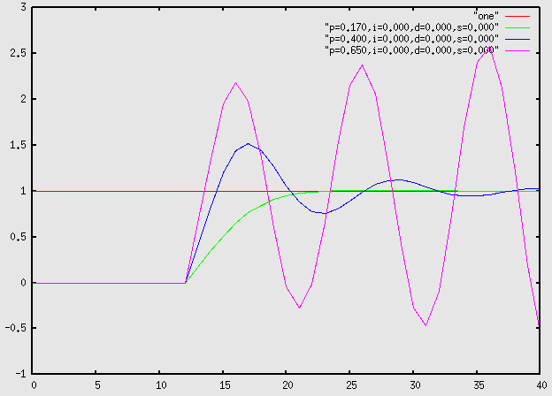
A control system that is improperly designed or adjusted incorrectly can become unstable. The typical results are wild oscillations of the output value that grow with time. The green line below represents a good control system. The blue line has severe overshoot, although it is still stable; note that the oscillations diminish with time. The purple line represents an unstable system; note that the oscillations increase with time. All three of these systems use a very simple proportional controller (in other words, the constants on the integral and derivative terms are zero). The only difference between the three systems is in the proportional gain (the nonzero constant on the proportional term).
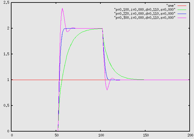
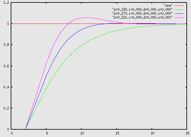
With a stable system, small adjustments to the proportional constant can still affect the speed and stability of the system. In this example, three closely related controllers are shown; one of the controllers has too much proportional gain (so it overshoots) one has too little (so it is slow) and one is "just right".
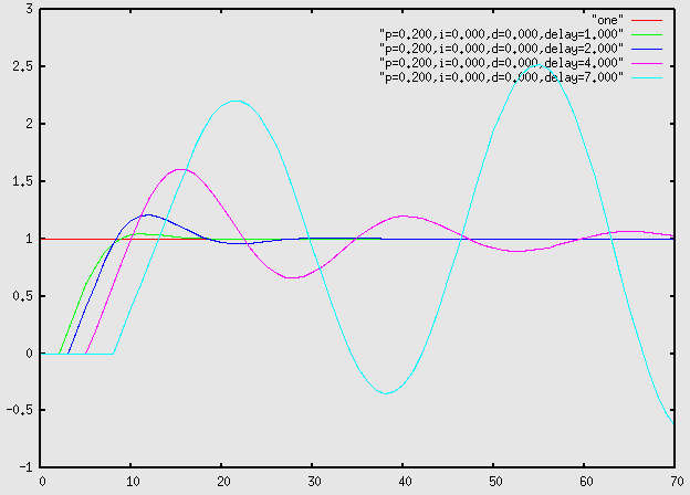
Almost all control systems have some delay in the control loop. Many factors introduce delay, including inertia in mechanical systems, finite response time of transducers, time needed for analog to digital or digital conversion, and computation time for digital controllers. The stability of a control system is often profoundly sensitive to the amount of delay in the control loop. The following example illustrates this. The four control systems show differ only in the amount of delay, which ranges from 1 to 7. With the smallest delay (delay=1, the green line), the system is pretty good; it reaches the desired value rapidly and it has only a tiny overshoot. With a delay of 2 (the dark blue line), the overshoot is significantly worse, and the system is also slower to respond. With a delay of 4 (the magenta line), the system is just barely stable; it oscillates and takes a number of cycles to settle. Finally, with a delay of 7, (the light blue line), the system becomes unstable, with growing oscillations.
Although powerful mathematical methods exist for the design of control systems, these generally require an accurate mathematical model of the target system. This can be difficult to obtain, particular when mechanical devices are involved with complex effects such as flexible components and friction. Thus, it is not unusual to construct a control system by taking an initial guess at appropriate parameters, observing the behavior of the system, and making adjustments as needed.
Here is some advice that is believed to be helpful (but that is not thoroughly tested!) for common situations that will arise with EECS 373 projects. First, try working with the integral and derivative terms set to zero and use the proportional term to adjust the system. If the system is unstable or if it shows oscillation or overshoot, try reducing the proportional term. If the system is stable but slow to respond, try increasing the proportional term. Once you have the proportional term set to the maximum value that does not produce oscillation or overshoot, look closely at the behavior of the system. If you observe steady state error, try introducing a small nonzero integral term. If the system seems to be slow to respond to changes, try introducing a small nonzero derivative term. If you introduce or change integral or differential terms, you will probably need to readjust the proportional term.
All of the examples used were produced with a simple
simulator written in Python:
www.python.org
The results are plotted with Gnuplot
www.gnuplot.info
If you want to play with it, the source code for the simulator is available here: simulator.py
It should work on most Unix systems, including the CAEN lab Linux and Solaris workstations. Both Python and Gnuplot are available for Microsoft Windows, but you're on your own for getting them installed!
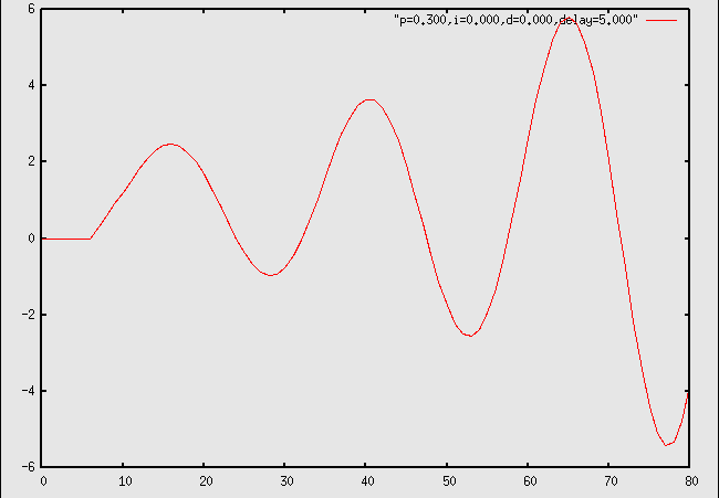
2. Assuming you cannot change the characteristics of the target system or change the total delay in the control loop, what would be the first thing you should try in order to fix this system?
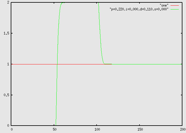
3. After following the advice in the answer to sample problem 2, the response of the system to a unit step is now this:
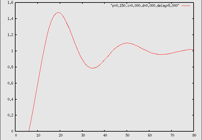
Is this a working control system?
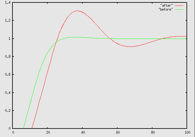
4. After considerable experimentation and long hours in the 373 lab, you get things into pretty good shape; the response of your control system looks like the green line in the plot below. The system smoothly and quickly approaches the desired value, with minimal overshoot or oscillation. Unfortunately, circumstances force you to replace the transducer and analog to digital converter on the transducer with very different ones. You are positive that the gain of your system has not changed at all, and careful measurements confirm this. Nevertheless, the response of the system now looks like the red line in the plot below. What probably happened?